ANN (artificial neural network)
Percepton
perceptron - 가장 간단한 인공 신경만 구조 중 하나임. perceptron은 층이 하나인 TLU(threshold logic unit)로 구성된다. 각 TLU는 모든 input(입력)에 연결되어있다.
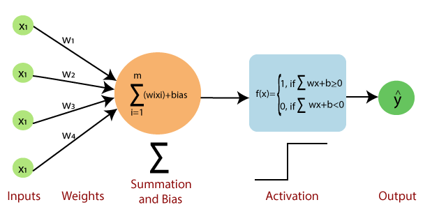
입력에 bias라는 편향값이 더해져서 다음과 같은 공식으로 perceptron이 표현된다.
w : vector of weights
x : vector of inputs
b : bias
φ : non-linear activation function.
Input data 로 위그림과 같이 TLU를 훈련시켜서 최적의 parameters (w1,w2,w3,w4)를 찾는다. 여기에서 weights는 각 corresponding input이 output에 대해 가지고있는 “importance”(중요도)를 의미한다.
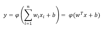
각 intput에 weight만큼 가중치를 설정해서 구한 이들의 sum이 특정 threshold보다 크면 function의 결과가 1, 보다 작으면 function의 결과가 0이 된다.
위 그림에서 보이는 바와 같이 bias라는 값을 통해 threshold 기준을 0으로 맞추어서 step function을 구현했다.
각 neuron을 activate할지 deactivate할지를 이 기준을 통해 설정할 수 있기때문에 이 단계는 활성화(activation) 함수라고 부른다.
weights와 threshold를 변경해서 각 input이 ouput에 얼마나 영향을 줄지를 제어하고 결국 model의 output을 제어할 수 있다. (You can think of the bias as a measure of how easy it is to get the perceptron to output a 1.)
Multilayer perceptron
single-layered perceptron으로는 non-linearity나 data의 complexity가 포함된 문제를 해결할 수 없다. 그래서 researcher들이 multilayer perceptron을 만들어서 여러개의 hidden layer를 구성하고 data속에 숨어있는 non-linearity를 찾아낸다.
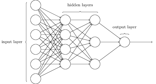
아래 그림과 같이 input layer(입력층)와 output layer(출력층)사이에 hidden layer(은닉층)가 존재한다.
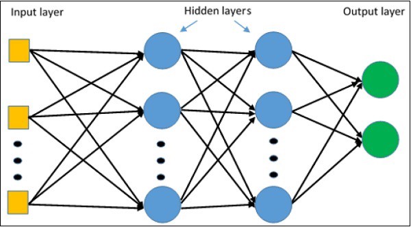
입력층과 가까운 층은 하위층(lower layers)이라고 부르고, 출력층과 가까운 층은 상위층(upper layers)이라고 부른다. 이렇게 은닉층을 여러개 쌓아 올린 인공 신경망을 심층 신경망 (Deep neural network)이라고 한다.
Multilayer perceptron은 intput-output pairs로 구성된 data set으로 훈련을 하면서 결국 input들과 output들사이의 dependencies (or correlation)을 model한다. 이 훈련과정에서 weights and biases와 같은 parameter들을 보정해서 model의 error를 최소화 한다.
Hidden layer들이 input data의 feature를 담고있다. 예를 들어서 MNIST data set를 입력해서 손글씨 숫자를 구분하는 model을 표현하는 neural network이 있다고 가정하면, 숫자 이미지의 특징들을 network가 학습하는 것이다.
각 layer가 어떤 내용을 담고 있는지를 다음 그림과 같이 표현할 수 있다.
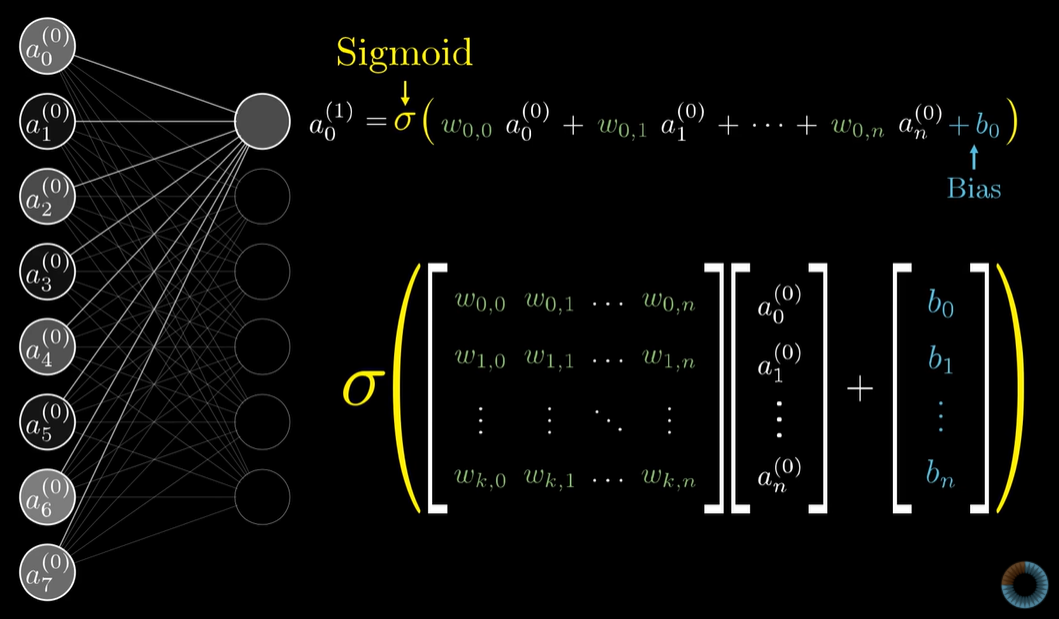
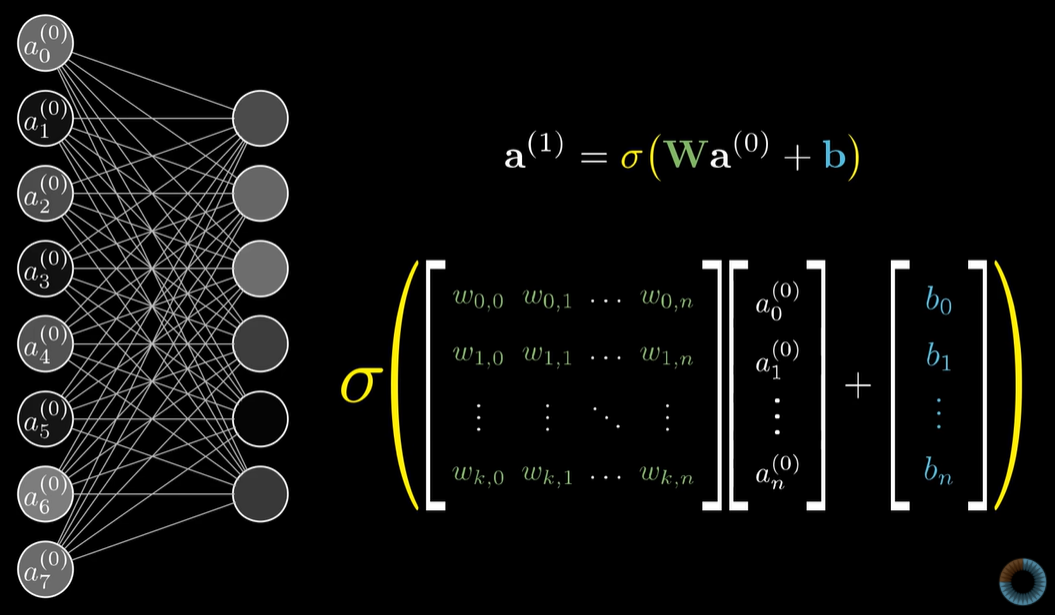
이전 layer의 neuron들의 output과 연결 가중치 값 w들을 가지고 다음 layer의 neuron을 계산하는 것이다. 연결 가중치 값 w는 matrix로, 이전 layer의 neuron output과 bias는 vector로 각각 표현할 수 있다. 그리고 sigmoid와 같은 활성화 함수를 통해서 neuron의 활성화 여부를 표현하도록 한다.
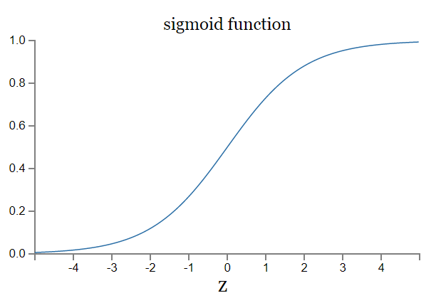
여기서 활성화 함수는 neural network의 output을 원하는 scale로 표현하도록 조정해주는 역할을 한다. 계단(step) 함수 또는 sigmoid 함수가 사용되는데, sigmoid는 계단 함수와 같이 0,1 으로 구분되는 binary가 아니라 0과 1 사이에서 어떤 값이든 가능하다. sigmoid는 small changes in weights and bias로 output에 small changes를 만들 수 있는 function이다.
sigmoid function:
간단하게 정리해보자면, 하나의 neuron을 input을 받으면 ouput을 내어주는 함수로 생각해볼 수 있다. 입력 data로 부터 output을 예측해내기위해 input과 ouput을 이어주는 network을 이 neuron들로 형성하고, 각 neuron들 간의 연결을 parameter값으로 조정한다. 더 정확한 output을 예측하기위해 parameter값의 최적화 과정을 거치게 된다.
Linear regression
아주 간단한 supervised learning중 하나인, linear regression문제에서 model의 parameter들이 어떻게 설정되는지 알아볼 수 있다.
다음과 같이 hypotheses h를 통해 output y를 예측하려한다면 linear 함수로 표현할 수 있다.
Input dataset에 두개의 features가 주어졌을 때, (x_0 =1)
input x와 output y를 mapping하는 linear 함수이고 여기에서 θ가 weights 또는 parameter를 의미한다. (위와 같은 공식에서 θi가 space of linear functions를 parameterize해서 x와 y의 mapping을 수행하기때문에 θ를 “parameter”라고 부른다.)
주어진 training data를 바탕으로 어떻게 적절한 parameter들을 찾을 수 있을까?
supervised learning에서는 우리가 y를 이미 알고있기때문에 y에 가장 가까운 h를 만드는 θ를 찾아볼 수 있다. Hypotheses h와 y의 차이를 계산하는 함수를 cost function J 라고 부르고 다음과 같이 정의한다. (input dataset에 총 n개의 samples/instances가 있고, ith번째 sample에 대한 예측값과 ground truth값의 차이를 계산하는 방식)
J는 linear regression에서 주로 사용되는 least-square cost function이고 이는 ordinary least squares regression model에서 cost function으로 사용된다. 우리는 J를 가장 최소화 시킬 수 있는 θ를 찾아야 한다.
gradient descent algorithm은 우리가 원하는 θ를 찾는 방법 중 하나이다. 처음 특정 값을 하나 guess를 해서 cost를 계산하고 이를 점차 줄여가는 방향으로 update를 반복적으로 진행하는 방법이다.
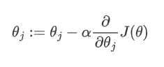
(여기에서 :=는 θ에 계산된 새로운 값을 assign하여 update한다는 것을 의미하고 α는 learning rate을 의미한다.) θ는 J가 가장 가파르게 감소하는 방향으로 update된다. 위 공식에서 cost function J의 partial derivative를 input x와 output y로 표현하면 다음과 같은 공식이 확인된다. 이런 방식을 LMS(“least mean squares”) update rule이라고 부른다.
parameter θ가 update되는 변화의 크기는 the error term (output y - hypothesis h)와 비례한다.
이렇게 θ를 반복적으로 update하여 최적의 값을 찾는 방법을 ‘‘경사하강법’‘이라고 한다.
경사하강법 Gradient descent
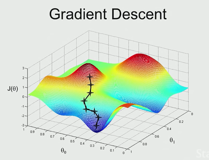
위 공식에서 설명한 것과 같이 경사하강법은 가중치(parameter)에 얼만큼의 변화를 주어야지 손실 함수 C(θ)를 (C for cost) 최소화할 수 있는지 알려준다.
다음 그림을 보면 가중치와 이 가중치들의 gradient cost function이 vector로 표현되어 있다. gradient of cost function은 어떤 방향으로 각각의 가중치 값이을 얼마나 움직여야 하는지를 알려준다. (w_0는 증가, w_1는 조금만 증가, w_2는 많이 감소, ….etc)

Gradient descent는 다음 그림과 같이 반복적인 계산을 통해 (미분 가능한) 해당 함수의 가장 낮은 위치를 찾아간다. 즉, 가장 정확한 output을 예측할 수 있는 최적의 θ 또는 parameter를 찾아주는것이다.
Gradient descent를 구현하는 방식을 간단하게 몇가지 얘기해보자면, gradient descent algorithm은 stochastic gradient descent(or incremental gradient descent)와 batch gradient descent로 두가지 방법이 존재한다.
Batch gradient descent는 매번 update를 진행할때에 entire training dataset를 모두 훌터보기 때문에 특히 training dataset이 크다면 속도와 cost가 나쁜편이다.
stochastic gradient descent는 random으로 dataset을 보기때문에 보통 cost function의 minimum에 근접하는 θ를 더 빠르게 찾는편이다. 그래서 training data set이 큰 경우에는 stochastic gradient descent를 선호하는 편이다.
역전파(back propagation)
model들이 어떻게 자신의 error/mistakes를 바탕으로 학습하는 과정은 두가지 방법으로 진행된다.
forward propagation(정방향 계산):
signal flow가 input layer에서부터 hidden layer를 통과하여 output layer까지 흘러간다. output layer의 decision은 ground truth labels를 기준으로 평가되고 output layer가 ground truth와 비교했을때에 얼만큼의 error(오차)가 발생했는지를 감지한다.
backward propagation(역전파):
model의 모든 parameter에 대한 network 오차의 gradient를 계산할 수 있다. 즉, 오차를 감소 시키기위해서 각 연결 가중치와 편향값이 어떻게 바뀌어야하는지를 찾는 것이다. gradient를 구하고나면 평범한 경사 하강법을 수행한다. 전체 과정은 network가 어떤 해결책으로 converge될때까지 반복한다.
forward + backward propagation은 간단하게 다음과 같이 진행된다:
-각 훈련 샘플에대한 역전파 알고리즘이 먼저 예측을 만들고 오차를 측정한다. (정방향 계산)
-역 방향으로 각 층을 거치면서 각 연결이 오차에 기여한 정도를 측정한다. (역방향 계산)
-감지된 error를 바탕으로 parameter θ들을 (e.g., weights와 bias) 보정한다. error가 감소하도록 가중치를 조정한다. (경사 하강법 단계)
상세 과정:
- 하나의 mini batch씩 반복적으로(iteratively) 진행해서 전체 훈련세트를 처리하며, 하나의 iteration을 epoch라고 부르는데, 각 mini batch는 network의 입력층으로 전달되어 첫번째 은닉층으로 보내진다. mini batch에 있는 모든 sample에 대해 해당 층에 있는 모든 뉴런의 출력을 계산한다. 계산된 결과는 다음 층으로 전달된다.
- 이런식으로 마지막 층인 출력증의 출력을 계산할때 까지 계속된다. 이렇게 정방향으로 진행하면서 중간 계산값을 모두 저장한다. (역방향 계산을 위해 저장)
- algorithm이 network의 출력 오차를 측정한다. (손실 함수를 사용해서 기대하는 출력과 network의 실제 출력을 비교하고 오차값을 반환한다.)
- 각 출력 연결이 이 오차에 기여하는 정도를 계산한다.(미적분의 가장 기본 규칙인 연쇄법칙을 사용해서 빠르고 효율적으로 진행한다.)
- algorithm이 또 다시 연쇄 법칙을 사용해서 이전 층의 연결 가중치가 이 오차의 기여 정도에 얼마나 기여했는지를 확인한다. 이런식으로 입력층에 도달할때까지 역방향으로 계속 반복한다. 이렇게 역방향 진행단계에서 오차 gradient를 거꾸로 전파함으로서 효율적으로 network에 있는 모든 연결 가중치에 대한 오차 gradient를 측정한다.
- 마지막으로 algorithm은 경사 하강법으로 방금 계산한 오차 gradient를 사용해서 network에 있는 모든 연결 가중치를 수정한다.
note: hidden layer의 연결 가중치를 random하게 초기화 하는것이 매우 중요함. 그렇지 못하면 훈련을 실패할 것임. 예를 들어 모든 가중치와 편향을 0으로 초기화하면 -> 층의 모든 뉴런이 같아진다. 따라서 역전파도 뉴런을 동일하게 바꾸어서 모든 뉴런이 똑같아진 채로 남고, 뉴런이 마치 하나인것처럼 작동하게 됨. 그래서 가중치를 random하게 초기화해서 대칭성을 깨고 역전파가 뉴런을 다양하게 훈련시키는 것임.
Normal equations
반드시 경사 하강법을 통해 반복적으로 parameter θ를 update하는 방식을 사용해야하는 것은 아니다. Parameter optimization을 위해 iteration없이 analytical 방식인 normal equation을 사용할 수 있다. Normal equation을 통한 optimization은 matrix를 사용하기때문에 multiple linear regression의 parameter를 한번에 계산해준다.
Normal equation 방식에서는 우리에게 주어진 input, output data set을 matrix형태로 다룬다.
matrix와 linear algebra를 사용해서 cost function J를 minimize하는 θ를 찾는다. 특히 소수의 features를 가진 dataset을 기반으로 model을 훈련하는 과정에서는 normal equation을 사용해서 더 빠르게 최적의 parameter θ를 찾을 수 있다.
Matrix의 특성 중 다음과 같은 특성을 사용하면,
cost function J와 J의 derivative를 다음과 같이 표현할 수 있다.
J의 derivative를 0으로 set해서 minimum cost function에 해당하는 parameter θ를 찾을 수 있다. matrix derivative 사용해서 얻을 수 있고 다음과 같이 찾은 θ를 normal equation이라고한다.
Normal equations are equations obtained by setting equal to zero the partial derivatives of the sum of squared errors or cost function; normal equations allow one to estimate the parameters of multiple linear regression.
Gradient descent vs. Normal equation
| Gradient Descent | Normal Equation | |
|---|---|---|
| In gradient descenet , we need to choose learning rate. | In normal equation , no need to choose learning rate. | |
| It is an iterative algorithm. | It is analytical approach. | |
| Gradient descent works well with large number of features. | Normal equation works well with small number of features. | |
| Feature scaling can be used. | No need for feature scaling. | |
| No need to handle non-invertibility case. | If (X^T X) is non-invertible , regularization can be used to handle this. | |
| Algorithm complexity is O(kn^2). n is the number of features. | Algorithm complexity is O(n^3). n is the number of features. |
Logistic regression
Regression에는 linear regression외에도 다른 유형의 문제들을 해결 할 수 있는 regression 기법들이 있다.
Types of regression:
- linear regression
- simple linear regression: predict output based on one feature
- multiple linear regression: predict output based on multiple features
- logistic regression
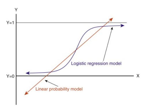
- binary: based on features, predict an output that is one of two possible classes (e.g., 0 or 1) logistic regression은 회귀이지만 확률값을 계산해서 분류를 하는 모델이다. used when the input data cannot be modeled by a linear regression line. (in other words, when we need non linearity to trace the data points & when applying linear regression wil result in outputs that are neither 0 or 1 which doenst fit into the givens scenario.)
- multinomial: based on features, predict an outputs that is one of many possible classes (i.e., multiple categories, two or more discrete outcomes) (e.g., predict what will be the most used transportation type in 2030 - possible outputs can be train, bus, tram, bikes.)
Logistic regression은 언제 사용할면 될까?
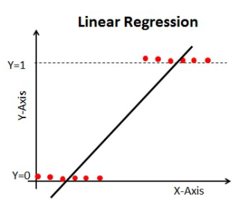
만약 주어진 input data로 0 또는 1이 되어야하는 output을 예측해야하는 문제가 있다면, 위 그래프와 같이 linear regression으로 modeling할 수가 없다. (regression line으로는 (0,1) range밖의 값이 output으로 나오기 때문에) 우리가 원하는 0 or 1의 output을 얻으려면 다음과 같이 sigmoid curve를 통해 예측 값을 찾을 수 있다.
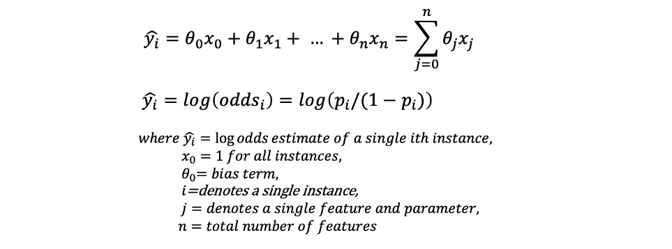
linear regression 문제를 해결할때와 동일하게 input feature와 parameter를 linearly combine하지만, linearly combined된 input과 parameter를 sigmoid function에 plug-in해서 probability(확률값)을 찾는다.
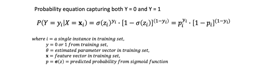
Binary logistics 문제의 경우 1 또는 0의 output을 얻을 확률을 표현해보면 다음과 같다.
x_i= single input instance (training set에서 하나의 observation)
y_i= 해당 instance의 output (0 or 1)
“p(y_i / x_i ; θ)” = ith x가 주어졌을때, θ로 parameterized 된 i번째 y의 distribution
odds = p / (1-p) 즉, probability of success divided by failure = P(success)/P(failure))
log-odds값은 linear regression function을 사용하여 estimate한 “y-hat”으로 표현된다. log-odds는 logit transformation으로도 불리며, linear form과 probability form 사이의 gap을 연결해주는 역할을 한다.
logit transformation이란? = odds or odds ratio의 log값으로 처리하는 tranformation. sigmoid function의 inverse이며 통계나 machine learning에서 data transformation을 위해 자주 활용된다. (https://en.wikipedia.org/wiki/Logit)
logistic regression model을 graph해보면, 다음과 같이 0와 1사이에서 continuous 값을 가진 function으로 확인할 수 있다.
주어진 data로 model을 하기위해 다음과 같은 순서로 변환해 나아간다: probability -> odds -> log-odds
이 셋을 monotonic relationship을 갖고있기때문에 (즉, probability increase-> odds increase -> log-odds increase) parameter를 estimate할 수 있다.
Likelihood (L(θ))
training set의 sample(or instance)마다 randomly estimated parameters θ를 사용해서 log odds를 계산한다. 그리고 sigmoid function을 통해 probability를 예측한다.
각 sample의 probabilities를 곱해서 likelihood를 찾을 수 있다.
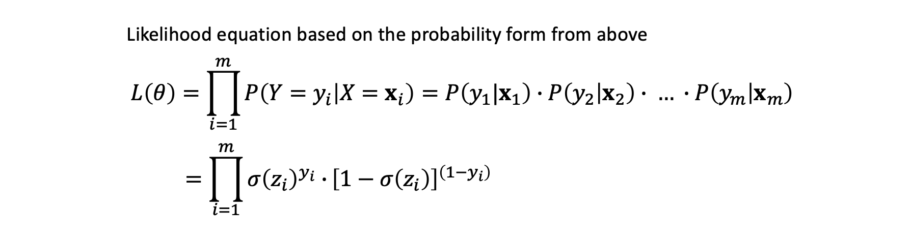
Likelihood를 maximize해서 optimal parameters로 converge할 수 있다. likelihood를 maximize해서 best parameter를 찾을 수 있다. 이 방식은 MLE(Maximum Likelihood Estimation)으로 불린다. maximum에 도달하게되면 처음 설정된 initial parameter값이 최적의 값으로 수렴된다. gradient descent/ gradient ascent와 같은 optimization algorithm으로 인해 이 수렴하는 과정이 진행된다.
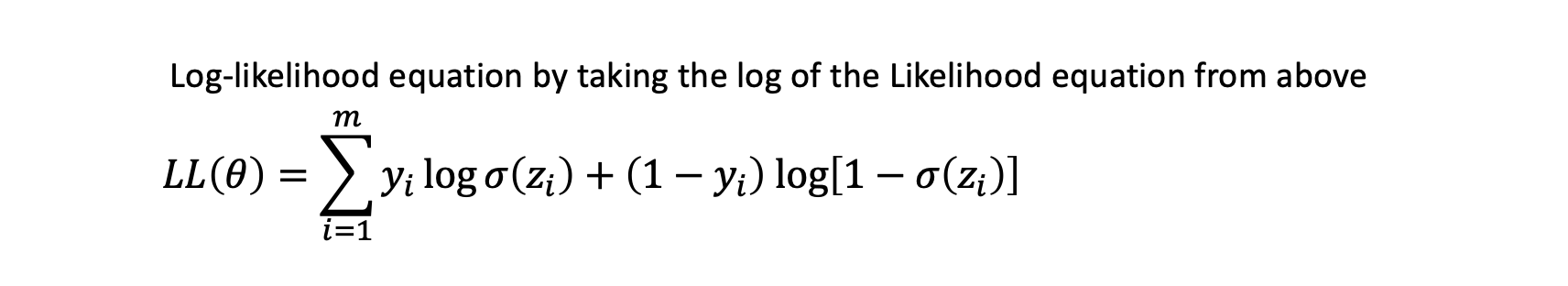
Likelihood의 maximum을 찾기위해 likelihood의 log을 활용한다. (probablilties와 같이 작은 scale의 값이 여러번 곱해지면 값이 너무 작아지기때문에 log를 활용) likelihood의 log를 계산하고 다음 log properties를 활용해서 summation operation으로 변환시킬 수 있다.
(log(XY) = log(X)+log(Y) and log(X^b) = b*log(X))
log of likelihood LL(θ)를 다음과 같이 계산한다.
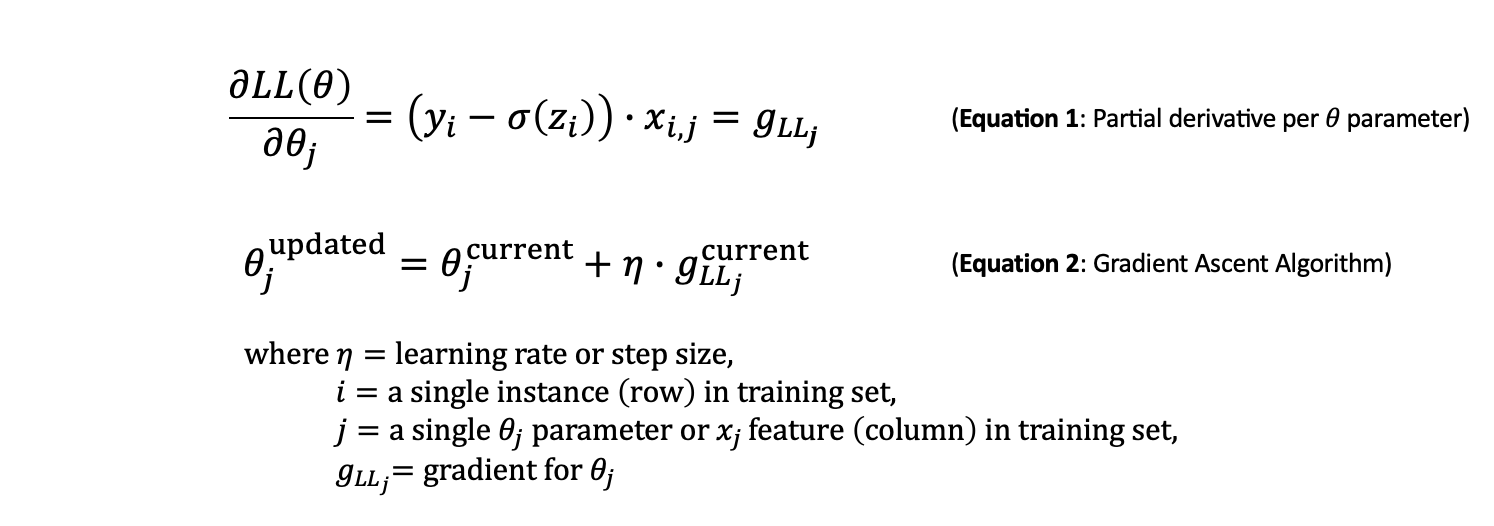
log-likelihood의 최대값을 찾기위해서 derivative를 활용한다. log-likelhood의 partial derivative를 (with respect to each θ)계산한다. 각 parameter의 gradient를 찾아서 optimal 방향으로 수렴하기 위한 방향으로 magnitude와 direction을 찾아간다.
linear regression때와 동일하게 learning rate (eta)으로 gradient ascent algorithm이 iteration마다 얼마나 큰 step으로 이동할지를 설정한다. (don’t want the learning rate to be too low, which will take a long time to converge, and we don’t want the learning rate to be too high, which can overshoot and jump around)
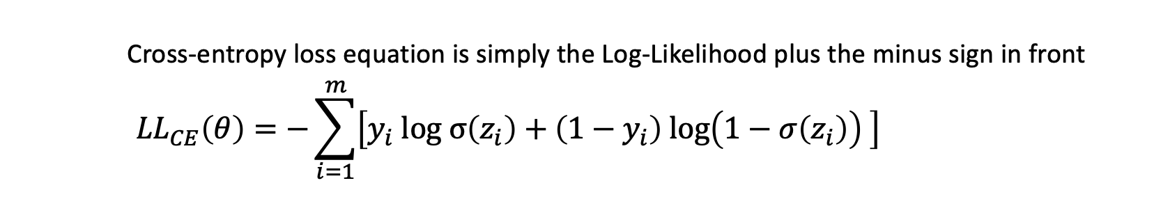
Cost Function
경사하강법을 통해 다음과 같은 cost function cross entropy loss equation을 최소화할 수 있는 최적의 parameter를 찾는다.
cost function의 partial derivative (with respect to parameter)를 활용하여 parameter들이 optimal될때까지 반복적으로 parameter를 update한다.
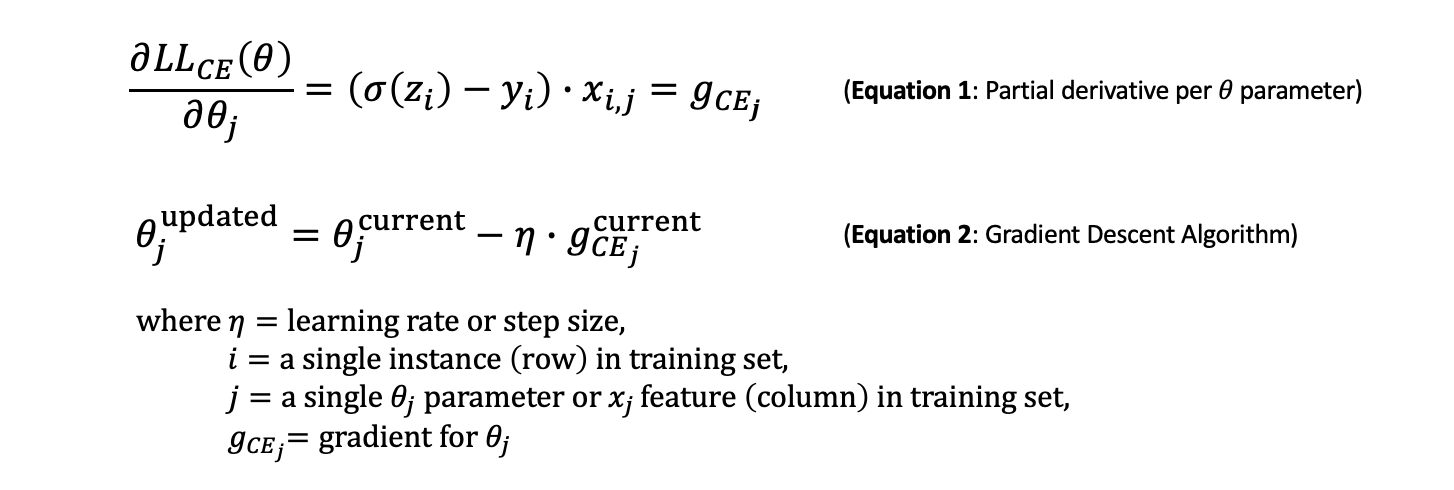
Cross entropy의 경우, convex graph이기때문에 gobal minimum을 보다 쉽게 찾을 수 있다.
Reference
- Geron, Aurelien. Hands on Machine Learning. O’Reilly, 2019
- deep neural network에서 network & parameter들의 역할 및 operation : https://www.youtube.com/watch?v=aircAruvnKk
- gradient descent explained : https://www.youtube.com/watch?v=IHZwWFHWa-w
- backpropagation explained with graphics : https://www.youtube.com/watch?v=Ilg3gGewQ5U
- normal equation in linear regression : https://www.geeksforgeeks.org/ml-normal-equation-in-linear-regression/
- logistic regression : https://towardsdatascience.com/understand-implement-logistic-regression-in-python-c1e1a329f460