Imbalanced Datasets
dataset에 분류하려는 class간의 balance가 맞지않는 경우를 imbalanced dataset이라고한다. (e.g. anomaly detection where 90% of dataset is normal and only 10% of dataset is abnormal. normal은 majority class, abnormal은 minority class로 불린다.)
imbalanced dataset을 handling할때에 preprocessing 단계에서 oversampling 또는 undersampling을 통해 balance를 강제로 맞추어서 데이터 분석 및 모델 훈련을 진행할 수도 있고, 또는 evaluating 단계에서 적당한 지표를 통해 정확하게 훈련된 모델의 성능을 평가할 수 있다.
Evaluating
precision & recall curve
high recall + high precision : the class is perfectly handled by the model
low recall + high precision : the model can’t detect the class well but is highly trustable when it does
high recall + low precision : the class is well detected but the model also include points of other classes in it
low recall + low precision : the class is poorly handled by the model
ROC and AUROC
| P(C | x) = probability of belonging to class ‘C’ when given ‘x’ |
| decision rule로 threshold T를 지정하고, P(C | x) ≥T 인 경우에만 ‘x’가 ‘C’로 분류된다. |
T=0이라면, 모든 ‘x’가 ‘C’로 분류되는것이고, T=1이라면, ‘x’는 model이100% confident할때에만 ‘C’로 분류되는것이다.
T=(0,1) range에서 각 T값이 false positive, true positive point를 생성한다. 이 point들을 모아서 graph over range of T하면 ROC curve를 얻을 수 있다. This curve starts at point (0,0), ends at point (1,1) and is increasing. A good model will have a curve that increases quickly from 0 to 1 (meaning that only a little precision has to be sacrificed to get a high recall).
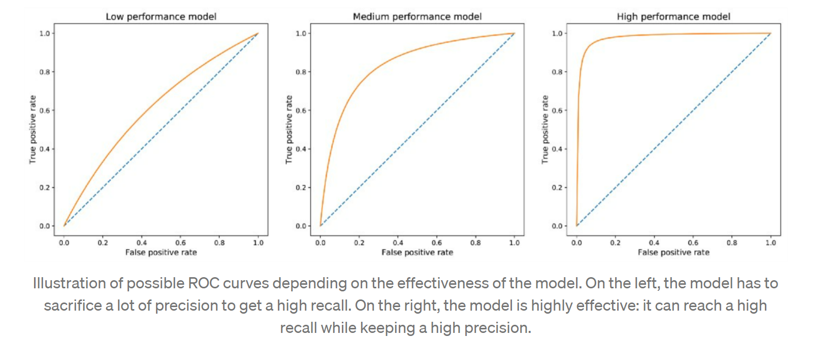
이 ROC curve를 기반으로 더 사용하기 편한 metric인 AUROC를 찾을 수 있다. AUROC = “Area Under the ROC curve” 이름 그대로 curve아래의 영역을 의미한다. AUROC값은 하나의 scalar값으로 ROC curve전체를 표현할 수 있다. AUROC가 1에 가까울수록 best case이고, 0.5에 가까울수록 worst case이다.
좋은 AUROC score는 model이 precision을 희생하지 않고도 좋은 recall을 얻을 수 있는 성능의 지표이다. imbalanced dataset에서 minority class에 대한 AUROC가 어느정도 확보되는지에 따라 모델의 성능을 판단할 수 있을 것이다.
Imbalanced data의 진짜 문제는 무엇인가?
imbalanced dataset의 example을 통해 graphically 살펴볼 수 있다.
imbalanced dataset contains: C0가 90%, C1이 10% portion을 차지하고, points from the class C0 follow a one dimensional Gaussian distribution of mean 0 and variance 4. Points from the class C1 follow a one dimensional Gaussian distribution of mean 2 and variance 1.
위 dataset의 distribution은 다음과 같다.
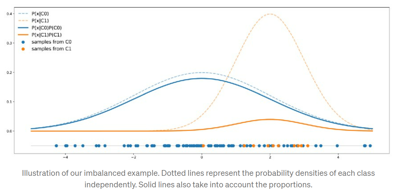
C0 curve가 언제나 C1 curve위에 위치한다. 어느 point이든 sample이 C0로 분류될 확률이 C1으로 분류될 확룔보다 높다는것을 의미한다. Bayes rule을 기반으로 수학적으로 표현하면 다음과 같다.

하나의 클래스가 (C0)가 항상 more likely than the other(C1).
이 dataset으로 classifier를 훈련시킨다면, classifier의 accuracy는 C0를 답할때에 가장 높을 수밖에 없다. 그래서 만약 highest possible accuracy를 얻는것이 classifier의 목적이라면, 이 imbalanced dataset은 문제가 되지 않는다. “should not be seen as a problem but just as a fact: with these features, the best we can do (in terms of accuracy) is to always answer C0. We have to accept it.”
dataset의 class들이 얼마나 separable한지도 중요한 사항이다.
Imbalanced dataset doesn’t necessarily mean that the two classes are not well separable. minority class를 분류하는데에 반드시 나쁜 성능을 가지는것도 아니다. 다음과 같은 예시를 보면,
For example, consider that we still have two classes C0 (90%) and C1 (10%). Data in C0 follow a one dimensional Gaussian distribution of mean 0 and variance 4 whereas data in C1 follow a one dimensional Gaussian distribution of mean 10 and variance 1.
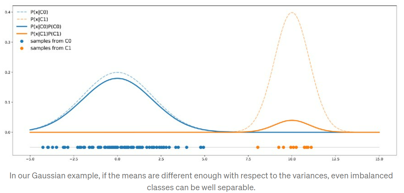
C0 curve가 항상 C1 curve위에 위치하지 않는다. there are points that are more likely to be drawn from class C1 than from class C0. In this case, the two classes are separated enough to compensate the imbalance. 이 경우에는 이런 imbalanced data로 훈련된 classifier도 minority class C1을 올바르게 분류할것이다.
Graphically, 각 클래스간의 separability에 따라서 error probability를 확인할 수 있다.
다음 그림은 not separable, slightly separable, well separable 세가지 case에서, 각 클래스별 분류 확률을 graph한것이다. dataset에는 하나의 feature와 두개의 분류 클래스가 있고 회색으로 칠해진 부분이 minimal error probability를 의미한다(given by the area under the minimum of the two curves).
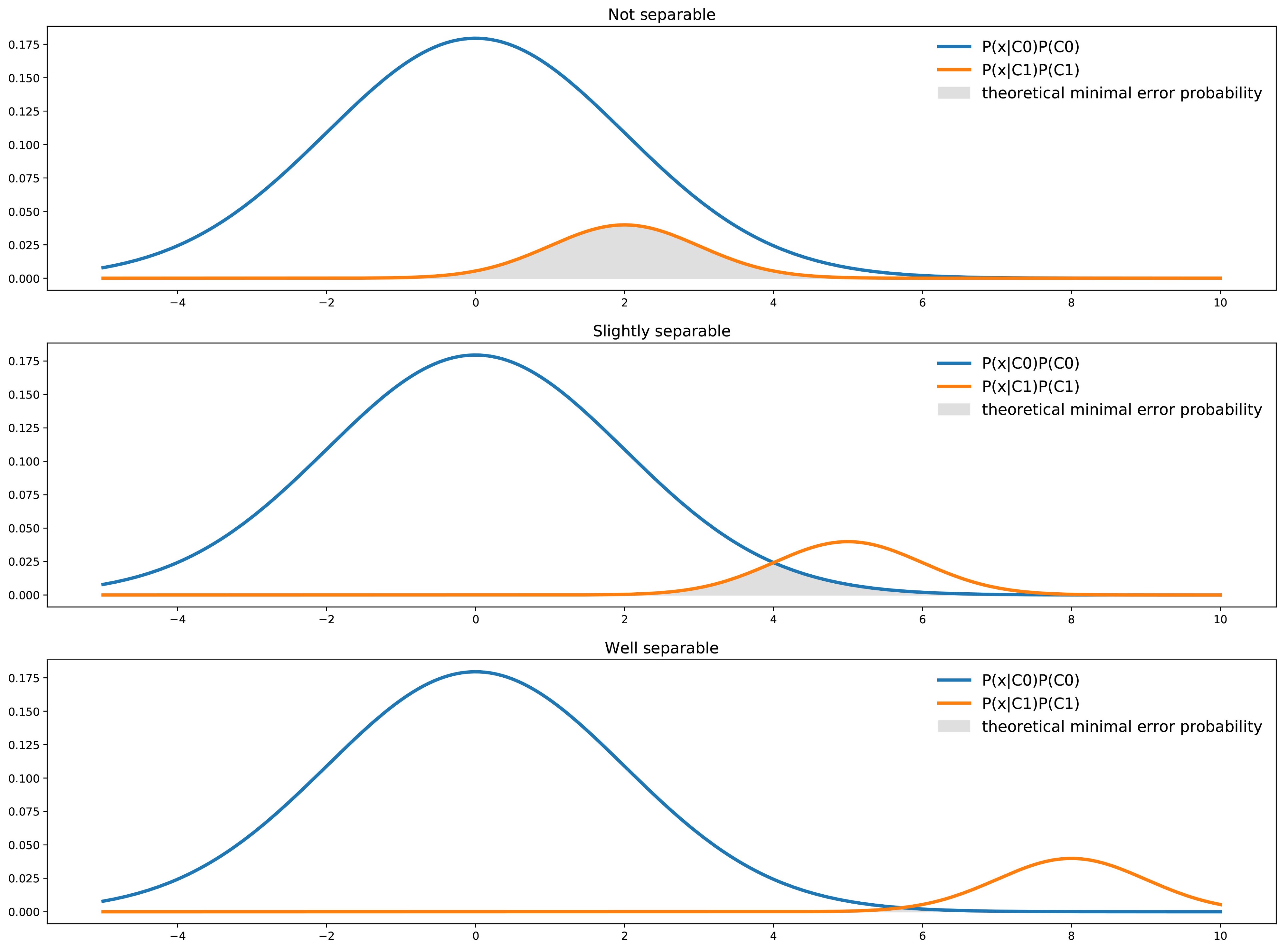
classifier는 각 point x에서 most likely of the two classes를 선택할 것이다. 각 point x에서 best theoretical error probability는 두개의 클래스 중 가장 less likely한 클래스로 부터 주어질 것이다.
그래서 overall error probaility는 area under the min of the two curves represented above.
Preprocessing
Re-sampling
over sampling
minority class내의 some point들을 replicate해서 minority class의 data size를 늘린다. (e.g., SMOTE() - synthetically made and prepared dataset)
Resampling
minority class에 있는 sample(관측치)를 random하게 replicate. 소수범주에 여러개의 동일한 sample들을 만들어서 minority쪽을 더 잘 학습하도록 변경하는 것 이다.
단순 copy하는 기법이지만, 경계선을 개선하는 효과가 크지 않음.
risk: minority class에 over fitting이 발생항 가능성이 있음.
SMOTE(synthetic minority oversampling technique)
가상의 데이터를 생성하는 방법. minority class 범주에서 가상의 samples을 만들어낸다.
k를 지정한다. (e.g., k=5, 임의로 선정한 minority sample 주변의 가장 가까운 neighbor k개를 선택한다.)
선택된 두 samples(관측치)에 다음 공식을 사용해서 가상의 관측치를 생성함.
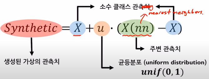
모든 minority 관측치에 대한 가상의 관측치를 생성함.
Borderline-SMOTE
SMOTE방식이지만, borderline 부분만 사용해서 over sampling하는 방식 임.
minority 범주 전체가 아닌, 경계부분에만 가상의 관측치를 생성함. 경계부분에만 집중하기때문에 분류경계를 향상하는대에 더 도움이 됨.
borderline을 찾는다.
minority class x_i에 대해 k개 주변 samples를 탐색 -> k개 sample들이 각각 majority vs. minority class중 어디에 belond하는지를 확인한다.
k개중에 majority class sample이 반이상이면 danger(borderline 영역의) 관측치로, 반이하라면 safe 관측치로, k개가 모두 majority class라면 noise 관측치로 판단함.
danger 관측치에 대해서만 SMOTE를 적용함.
ADASYN (Adaptive synthetic sampling approach)
sampling하는 개수를 위치에 따라 다르게 설정함.
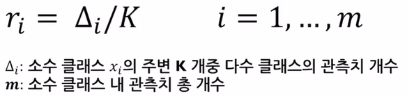
r_i(majority class 관측치의 비율)는 minority class sample이 majority class 범주 기준으로 어디에 위치하는지를 표현하는 값이다. 즉, r_i는 각 minority class sample주변에 얼마나 많은 majority class sample들이 있는지를 정향화한 지표임.
모든 minority class sample에 대해 주변을 k개 만큼 탐색하고 그중 majority class 관측치의 비율을 계산함 -> r_i
계산한 r_i값을 scaling함. (r_i값을 모두 더해서 각 r_i값을 그 sum으로 나누어줌.)
G = majority class 개수 - minority class 개수.
모든 r_i값에 G를 곱한다. r_i의 정도에 따라 생성되는 sample의 수가 다르게 됨.
(주변에 majority class sample들이 대부분인 경우에는 r_i값이 높고, 더 많은 가상의 minority sample이 생성될것임. minority class 주변의 majority class의 수에 따라 유동적으로 가상sample의 생성이 가능해짐.)
각 minority class를 seed로 하여 할당된 개수 만큼 SMOTE를 적용
under sampling
majority class내에서 sampling을 통해 부분적으로만 sample point들을 사용해서 majority class의 data size를 줄인다.
Random undersampling
majority class에 있는 samples(관측치)를 random하게 eliminate
risk: random하게 제거하기때문에, sampling할때마다 분류 경계선이 달라지고, 분류 모델의 성능이 달라질 수 있다.
Tomek links
majority & minority classes 사이를 탐지하고 정리를 통해서 부정확한 분류 경계선을 방지한다.
tomek link = i번째 sample(a point in majority class)과 j번째 sample(a point in minority class)사이에 아무런 sample이 위치하지 않는 경우, 이 둘이 tomek link를 형성한다고 한다. 둘 중 하나는 noise이거나 둘다 경계선 근처에 있음. majority와 minority경계 영역의 pair들을 찾기위해 사용됨.
Tomek link 형성 후, majority class에 속한 관측치를 제거해서 두 class간의 경계선을 찾는다. 경계 영역에서의 majority class의 sample들이 제거되었기때문에 분류경계선이 majority class에 덜 편향된 상태로 향상됨.
CNN (Condensed Nearest Neighbor Rule)
majority & minority classes의 경계 영역의 majority class samples만 남기고 나머지를 제거하는 undersampling기법. 경계영역에만 condense된 상태로 두 class를 나눈는 경계선을 찾는다.
CNN 과정:
1) minority 범주 전체와 majority 범주에서 무작위로 하나의 sample을 선택하여 sub data를 구성한다. 2) 그 하나의 sample을 1-NN (“one-Nearest Neighbor”) 알고리즘을 통해 분류한다. 해당 sample과 가장 가까운 관측치를 majority 범주에서 하나, minority 범주에서 하나를 찾아서 더 가까운 class로 변환시킨다. 3) majority로 분류된 관측치를 제거한다. 4) 줄어든 majority sample을 가지고 분류 경계선을 찾는다.
One-sided selection (OSS)
Tomek links + CNN
위와 같은 방법들을 통해 partially or fully dataset을 rebalancing한다. in what proportions should we rebalance?
dataset에서 class들의 portion을 하나의 중요 정보이다.
Resampling을 통해 dataset내의 proportion이 변동되면, we show the wrong proportions of the classes to the classifier model during the training. Resampling된 dataset으로 학습한 classifier 모델은 변동없이 original dataset으로 훈련한 model 대비, future real test data로 검증했을때에 낮은 accuracy를 얻을 것이다.
Resampling method는 dataset의 “reality”를 변동시키는 것이기 때문에 classifier의 목적에 따라 portion을 조정할지 고민해서 cautiously 적용해야한다.
만약 두개의 class를 가진 imbalanced dataset에서 two classes가 well separable하지 않고 best accuracy를 목적으로 classifier를 만든다면, 하나의 class만 답으로 찾는 classifier이라도 문제가 되지는 않을것이다.
getting additional features
dataset의 portion을 조정하기보다, additional feature를 추가하여 이를 통해 class들간의 separability를 증가시킬수 있다. (find a new additional feature that can help distinguish between the two classes and, so, improve the classifier accuracy.)
modeling 조정
cost-based classification (cost sensitive learning)
false positive와 false negative가 현재 classification 문제에서 정확하게 어떤 consequence를 가지고, 얼만큼의 cost을 발생시킬 지를 고민해보아야한다. errors are not necessarily symmetric.
Consider then more particularly that we have the following costs:
- predicting C0 when true label is C1 costs P01
- predicting C1 when true label is C0 costs P10 (with 0 < P10 « P01)
objective function을 redefine한다. classifier의 목적은 best accuracy가 아닌, lower prediction cost가 된다.
theoretical minimal cost
expected prediction cost를 최소화하는 방식으로 다음과 같이 classifier의 objective function을 설정한다.

References
“Handling imbalanced dataset in machine learning Deep Learning Tutorial 21 (Tensorflow2.0 & Python)” by codebasics : https://www.youtube.com/watch?v=JnlM4yLFNuo - “[핵심 머신러닝] 불균형 데이터 분석을 위한 샘플링 기법” by : [김성범 소장] https://www.youtube.com/watch?v=Vhwz228VrIk&list=PLpIPLT0Pf7IoTxTCi2MEQ94MZnHaxrP0j&index=7
- “Handling imbalanced datasets in machine learning” by Baptiste Rocca from https://towardsdatascience.com/handling-imbalanced-datasets-in-machine-learning-7a0e84220f28
- “7 Techniques to Handle Imbalanced Data” from https://www.kdnuggets.com/2017/06/7-techniques-handle-imbalanced-data.html
- “The 5 Most Useful Techniques to Handle Imbalanced Datasets” from https://www.kdnuggets.com/2020/01/5-most-useful-techniques-handle-imbalanced-datasets.html