How backpropagation works in Pytorch

Neural network은 단순하게 function이다. 원하는 result를 output으로 만들어 낼 수 있도록 아주 delicate하게 tweak된 (or 훈련된) composite mathematical function이다. 이 훈련과정은 backpropagation이라는 알고리즘을 통해서 수행된다. Backpropagation은 network의 input weights에 대한 loss의 gradient (즉, gradients of the loss with respect to the input weights)를 계산해서 결국 loss를 줄일수 있는 방향으로 weights를 update한다.

neural network을 개발하는 과정은 간략하게 다음과 같다.

1. model architecture 정의
2. input data를 넣고 forward propagate on the architecture
3. loss값 계산
4. Backpropagation (각 weight를 위한 gradient를 계산한다.)
5. learning rate을 사용하여 조절된 만큼 weights 값을 update한다.

Input weight의 작은 변화에 따른 loss 값의 작은 변화를 그 weight의 gradient라고하고, gradient는 backpropagation을 통해 계산된다. 위 과정이 반복적으로 진행하면서 loss값을 최소화 할 수 있는 weights를 가진 network을 찾을 수 있다.

각 iteration마다 여러 gradients가 계산되고, computation graph가 생성되어서 gradient functions를 저장해준다. Pytorch의 경우에는 Dynamic Computation Graph(DCG)를 생성한다. 매번의 iteration마다 DCG는 새로 생성되어서 (built from scratch), gradient calculation에 최대한의 flexibility를 제공한다.

Forward operation인 Mul function의 경우 MulBackward 라는 backward operation이 있고, 이것은 backward graph에 dynamically integrate되어서 gradient를 계산하는 역할을 수행한다.

Autograd

Pytorch autograd 클래스는 derivative(i.e., Jacobian-vector product)를 계산하는 역할을 수행한다. autograd는 gradient enabled tensor에 수행되는 operations의 graph를 기록하고 acyclic graph인 DCG를 생성해준다. graph의 leaves = input tensors, graph의 roots = output tensors. Gradients는 graph를 root에서부터 leaves까지 trace하면서 계산된다. (multiplying every gradient via chain rule)

Pytorch autograd documentation

DCG (Dynamic Computational Graph)

gradient enabled tensors (variables), functions (operations) 가 함께 dynamic computational graph를 구성한다. data와 data에 적용되는 operations의 flow는 runtime에 정의되기때문에 computational graph는 dynamic하게 만들어진다. Pytorch의 autograd가 이 graph를 만드는 역할을 수행한다.

simple DCG for multiplication of two tensors:

(초록 박스= variable, 보라색 박스= operation)

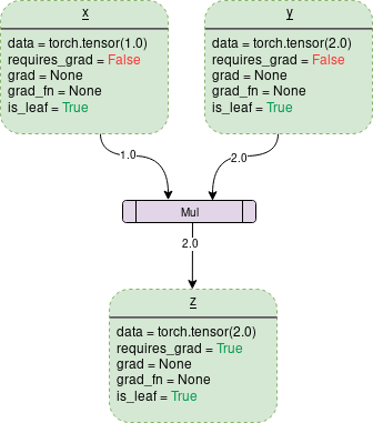
각 variable object는 다음과 같은 members를 가지고있다.

data: variable이 가지고있는 data. 위 그림에서 x는 1 by 1 tensor를 가지고있고 그 값은 1.0 이다.

requires_grad: boolean 값을 가진다. True일 경우 모든 operation history를 track하고, gradient computation을 위해 backward graph를 만든다.

grad: gradient의 값을 가진다. 만약 requires_grad가 False라면, grad는 None을 가진다. requires_grad가 True이더라도, .backward() 함수가 호출되지 않았다면 grad의 값은 아직 None이다. 예를 들어서 variable=out을 사용해서 out.backward()를 진행한다면, x.grad()는 ∂out/∂x (gradient of “out” with respect to x)

grad_fn: gradient를 계산하기위해 사용되는 backward function

is_leaf: node가 leaf인 경우는 다음과 같다:

1. node가 x=torch.tensor(1.0) 또는 x=torch.randn(1,1)와 같은 function을 통해서 explicit하게 initialize됨.
2. requires_grad=False를 가진 tensors에 opertions를 수행한 후 생성된 node.
3. some tensor에 .detach() 함수를 호출하여 생성된 node.

.backward()를 호출함으로써, requires_grad와 is_leaf에 True를 가진 node들만 gradients를 가지게 된다. (Gradients are of the output node from which .backward() is called, w.r.t other leaf nodes.)

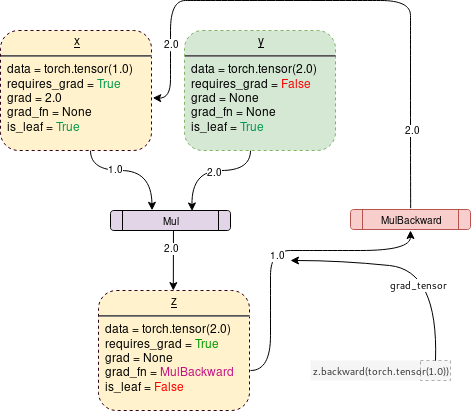
requires_grad=True로 설정되면, 다음 그림과 같이 Pytorch는 operation을 tracking하기 시작하고, gradient functions을 저장한다.

# code to generate graph above
import torch

# Creating the graph
x = torch.tensor(1.0, requires_grad = True)
y = torch.tensor(2.0)
z = x * y

# Displaying
for i, name in zip([x, y, z], "xyz"):
    print(f"{name}\ndata: {i.data}\nrequires_grad: {i.requires_grad}\n\
grad: {i.grad}\ngrad_fn: {i.grad_fn}\nis_leaf: {i.is_leaf}\n")

neural network의 훈련이 완료되었거나, network의 성능을 확인할때에는 더이상 operation의 history를 tracking하지 않아도되고, backward graph를 생성하지 않아도된다. 그럴때에는 다음 코드와 같이 .no_grad()를 호출하여 gradient tracking을 더이상 하지 않고 code를 더빠르게 실행 할 수 있도록 지정할 수 있다.

import torch
# Creating the graph

x = torch.tensor(1.0, requires_grad = True)
# Check if tracking is enabled
print(x.requires_grad) #True
y = x * 2
print(y.requires_grad) #True

with torch.no_grad():
	# Check if tracking is enabled
	y = x * 2
	print(y.requires_grad) #False

backward() 함수

backward() 함수는 root tensor에서부터 모든 traceable leaf node까지 backward graph를 통해서 gradients의 arguments(기본적으로 1x1 unit tensor)를 pass해서 gradients를 계산한다. 계산된 gradient는 각각의 leaf node의 .grad에 저장된다.

forward pass동안 backward graph는 이미 dynamically 만들어졌기때문에 backward function은 이 graph를 사용하여 gradient를 계산하고 저장만 하면 된다.

import torch
# Creating the graph
x = torch.tensor(1.0, requires_grad = True)
z = x ** 3
z.backward() #Computes the gradient 
print(x.grad.data) #Prints '3' which is dz/dx 

z.backward()가 호출된다면, tensor가 자동으로 z.backward(torch.tensor(1.0))로 pass된다. 여기에서 torch.tensor(1.0)은 chain rule gradient multiplications를 terminate하기위해 제공된 external gradient이다. 이 external gradient는 MulBackward에게 input으로 전달되어서 x의 gradient를 계속해서 계산한다. .backward()에 전달된 tensor의 dimension는 gradient가 계산되고있는 tensor의 dimension과 동일해야한다. 예를 들어보면,

Example)

Gradient enabled tensor x and y와 어떤 함수 z가 다음과 같이 정의된다면,

x = torch.tensor([0.0,2.0,8.0], requires_grad = True)
y = torch.tensor([5.0,1.0,7.0], requires_grad = True)
z = x * y

x 또는 y의 관점에서 z의 gradient (1x3 tensor) 를 계산하려면 (in order to calculate gradients of z wrt x and y), external gradient가 z.backward() 함수로 전달되어야 한다.

z.backward(torch.FloatTensor([1.0, 1.0, 1.0]))

그냥 z.backward() 를 호출한다면, 다음과 같은 에러가 발생 - RuntimeError: grad can be implicitly created only for scalar outputs.

Backward function으로 전달된 tensor는 weighted output of gradient의 weights와 같다. 수학적으로는 Jacobian matrix of non-scalar tensors로 multiply된 vector이다. 그래서 거의 항상 backward가 호출된 tensor와 동일한 unit tensor의 dimension이어야한다 (unless weighted outputs need to be calculated.)

Jacobians and vectors

Pytorch의 autograd 클래스는 간단하게 설명하자면 Jacobian-vector product를 계산하는 engine이다. Jacobian matrix는 matrix representing all the possible partial derivatives of two vectors이다. (즉, the gradient of a vector with respect to another vector)

실제 process에서 Pytorch는 Jacobian 전체를 모두 계산하지는 않고 더 간단하고 효율적인 방식으로 JVP(Jacobian Vector Product)를 직접 계산한다고 한다.

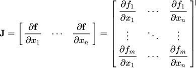
수학적으로 계속 설명을 해보자면, vector X=[x1, x2, …, xn]을 사용해서 함수 f를 통해 다른 어떤 vector f(X) = [f1, f2, …, fn]을 계산한다면, Jacobian matrix(J)는 다음과 같이 partial derivative combination들을 가지고있다.

gradient of f(X) with respect to X in matrix form:

만약 Pytorch gradient enabled tensors X가 다음과 같다면,

X = [x1, x2, …, xn] (=the weights of some ML model)

X undergoes some operations to form a vector Y = f(X)

Y = f(X) = [y1, y2, …, ym] (=the targets of some ML model)

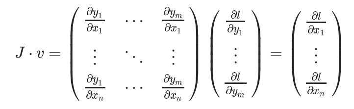
그 다음 Y가 사용되어서 scalar loss L을 구한다. (Suppose a vector v is the gradient of the scalar loss L with respect the vector Y)

여기에서 vector v는 grad_tensor이고, backward() function에 argument로 전달된다.

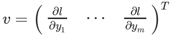
우리가 ML model의 훈련에서 찾고자하는 “loss L with respect to the weights X”를 계산하기위해서 다음과 같이 Jacobian matrix J를 vector v와 vector-multiplication을 수행한다.

References

1. PyTorch Autograd: Understanding the heart of PyTorch’s magic by Vaibhav Kumar
2. https://medium.com/towards-data-science/pytorch-autograd-understanding-the-heart-of-pytorchs-magic-2686cd94ec95
3. Backpropagation https://ml-cheatsheet.readthedocs.io/en/latest/backpropagation.html
4. PyTorch Autograd Explained - In-depth Tutorial by Elliot Waite https://www.youtube.com/watch?v=MswxJw-8PvE